Calculating the Confidence Interval: The Bootstrap method
發布時(shí)間:2017-09-18 | 來(lái)源:
作者:石川
1 Start with t-distribution
Parameter estimation is everywhere in quantitative investment. As an example, we must provide estimate of mean and variance of assets in the Markowitz's mean-variance framework of asset allocation. In most of the cases, having only the point estimate of a parameter of interest is insufficient. We are more interested in the error between our estimate and the true value of that parameter from the unknown population. In this regard, interval estimate -- in particular the confidence interval of the parameter -- provides the information we demand.
People are most familiar with the confidence interval (CI) for the population mean. With the Central Limit Theorem and the Normal distribution assumption, there is an elegant expression for the CI of the population mean. Specifically, one can convert the sample mean to a t-statistic using the sample standard deviation, and then find the critical values by looking up the t-value table. With the critical values, it is very easy to calculate the CI. Since Student's t distribution is symmetric, the CI computed this way is also symmetric.
Let's refer to the method described above as the traditional method from Normal Theory. I'd like to talk more about the two strong assumptions behind it: the Central Limit Theorem and the Normal distribution.
Suppose that the population satisfies the Normal distribution and we want to find the CI of its mean. If σ -- the standard deviation of the population -- is known, then we can use Normal distribution to compute the CI. If, on the other hand, σ is unknown, then we must use s -- the standard deviation of the sample -- to replace σ and use t-distribution to replace Normal distribution in the calculation of the CI. This is the intention for the t-distribution to be developed. Therefore, using t-distribution to compute CI requires the population to be normally distributed.
However, for most problems in practice, the population is far from normally distributed and it seems that this prevents us from using t-distribution. The good news is that we have another powerful weapon in our arsenal, the Central Limit Theorem. It says that no matter what the distribution of the population looks like, that of the population mean is asymptotically approaching to Normal. As a result, we can still use the t distribution to compute its CI.
In probability theory, the central limit theorem establishes that, in most situations, when independent random variables are added, their properly normalized sum tends toward a normal distribution (a bell curve) even if the original variables themselves are not normally distributed. The theorem is a key concept in probability theory because it implies that probabilistic and statistical methods that work for normal distributions can be applicable to many problems involving other types of distributions.
The argument above indicates that we heavily rely on the Central Limit Theorem and the Normal distribution assumption when calculating the CI for the mean. However, if the population distribution is very irregular or if the sample size is far from enough, the normal approximation of mean from the Central Limit Theory can be very questionable and the CI calculated using the t distribution can be inaccurate.
Other than mean, we are also interested in other statistics such as the median, the percentiles, the standard deviation, the correlation coefficient, just to name a few. Unlike the mean, there exists no elegant expression from which their CIs can be computed nicely. As a result, their CIs cannot be computed by the trandition method based on the Normal Theory.
To conquer these difficulties, this article introduces a statistical technique named Bootstrap and we will show that it is very powerful in computing the CI for various statistics.
2 Bootstrap: The origin and principle
The bootstrap is a computer-based method for assigning measures of accuracy to statistical estimates. -- Efron & Tibshirani, An introduction to the bootstrap, 1993
Bootstrap was popularized by Bardley Efron in 1979 and he also coined the term 'Bootstrap'. The key idea behind it is to perform computations on the data itself to estimate the variation of statistics that are themselves computed from the same data. Modern computing power makes Bootstrap very simple to implement. Bootstrap comes from the English phrase 'pull yourself up by your bootstraps', which means that one must lift himself up the ground by pulling his bootstrap. What it implies is that 'you should improve your situation by your own efforts'.
In the context of parameter estimation, Bootstrap means we can only use the data at hand, without making any assumption about the population, to measure the error of the sample statistics when they are used as the estimates of the true yet unknown population statistics.
The central idea is that it may sometimes be better to draw conclusions about the characteristics of a population strictly from the sample at hand, rather than by making perhaps unrealistic assumptions about the population. -- Mooney & Duval, Bootstrapping, 1993
So what shall we do specifically? How do we estimate the error of the statistics obtained from the sample data just by using the same data at hand (again and again)? To answer this question, we must talk about a very important technique first: resampling with replacement. Here, 'with replacement' is the key. To explain it, think about the following example. Suppose a jar contains 10 balls labelled from 1 to 10, and we draw balls from the bag one at a time. Suppose we get No. 3 ball in the first draw. 'Resampling with replacement' requires we put it back into the jar before the next draw. As a consequence, in the second draw, we are equally likely to draw any of the 10 balls, including No. 3 ball. In contrast, there are many 'resampling without replacement' in our daily life, such as the 36/7 lottery and the World Cup draw. In those circumstances, the balls won't be put back once they are drawn from the pool.
With this technique in mind, we are now ready to explain the Bootstrap principle. We start with the following setup:
1. Let v represent a populate statistic of interest (e.g., it can be the mean, the median, the standard deviation, etc) from the unknown population distribution F.
2. Let x1, x2, …, xn be a sample from the population. We refer to it as the original sample.
3. Let u represent the sample statistic corresponding to v.
4. Using the data in the original sample as our new 'population', conduct resampling with replacement to derive a Bootstrap sample. The data in the Bootstrap sample is denoted by x1*, x2*, …, xn*. The Bootstrap sample's size must be the same as the size of the original sample.
5. Let u* be the Bootstrap statistic computed from the resample.
Bootstrap principle says: The variation of u (around v) is well-approximated by the variation of u* (around u). To determine the variation of u*, we conduct resampling with replacement using the original sample data to derive a large number of Bootstrap samples (without the power of a modern computer, this could be a mission impossible for a human being). We compute the statistic u* from each of these samples and they constitute the distribution of u*. Using this distribution, it is easy to tell how u* varies around u, and we use this to approximate how u varies around v. The variation of the statistic u will depand on the size of the original sample. Therefore, if we want to approximate this variation we need to use Bootstrap samples of the same size. With the Bootstrap principle, we can use the empirical Bootstrap method to compute the confidence interval of any statistic.
3 Empirical Bootstrap method
We use a 'toy example' to explain how to find the CI for the population mean using the empirical Bootstrap method. Suppose we have the following 10 sample data from an unknown population: 30, 37, 36, 43, 42, 48, 43, 46, 41, 42. There are two questions to be addressed: (1) find the point estimate of the mean; (2) find the 80% Bootstrap confidence interval. Since the sample mean is the point estimate of the population mean, the answer to the first question is straightforward and it is 40.8. As for the second question, since the sample size is small and we have no knowledge about the distribution of the population, we use the empirical Bootstrap method, rather than the tranditional method, to find the CI.
To find the CI we need to know how much the distribution of sample mean, \bar x, varies around the population mean, μ. In other words, we would like to know the distribution of δ = \bar x – μ. δ is the error when we use \bar x to estimate μ. If we knew the distribution of δ, we could find the critical values that are required to compute the CI. In this example, since we want to derive the 80% CI, the critical values are δ_{0.9} and δ_{0.1}, the 10% and 90% percentile critical values of δ. With these the confidence interval is then,
The reasoning behind this is,
We hasten to point out that the probability computed above is conditional. It represents the probability that the variation of the sample mean \bar x around the true mean μ is between δ_{0.1} and δ_{0.9}, given that the true mean is μ. Unfortunately, since there is only one sample from the population and the true mean μ is unknown, we don't have the distribution of δ, and therefore we don't know the values of δ_{0.9} and δ_{0.1}. However, we do have the Bootstrap principle. It says even though we don't know how \bar x varies around μ (i.e., the distribution of δ), it can be approximated by how \bar x* varies around \bar x, i.e., the distribution of δ*, where δ* is the difference between the Bootstrap statistic and the sample statistic,
Since δ* is computed by resampling the original data, we can have a computer simulate δ* as many times as we'd like -- from each Bootstrap sample, we find its mean and subtract the original sample mean (40.8) from it. By the law of large numbers, we can estimate the distribution of δ* with high precision. We find the critical values δ*_{0.9} and δ*_{0.1} from the distribution of δ*, and use them as the approximation of δ_{0.9} and δ_{0.1}. The CI of μ then follows,

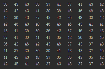
The procedure above shows the power of the empirical Bootstrap method. Back to the example, 200 Bootstrap samples are generated with the help of a computer program. The figure below shows 10 of them (one resample in each column).
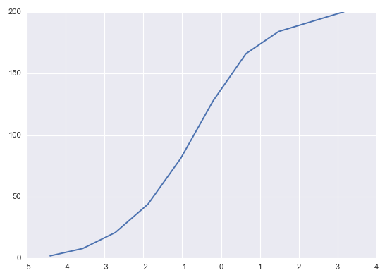
With these resamples, we find 200 values of δ* who ranges from -4.4 to 4.0. Its cumulative density function looks like the following.
Next, we need to find out δ*_{0.9} and δ*_{0.1} from these values. To do this, we sort these 200 δ* in an ascending order. Since δ*_{0.9} is the 10th percentile we choose the 20th element in the list. Likewise, since δ*_{0.1} is the 90th percentile we choose the 181st element in the list. They are δ*_{0.9} = -1.9 and δ*_{0.1} = 2.2. Recall that the sample mean is 40.8, and therefore the 80% confidence interval for μ is,

4 Bootstrap percentile method
Let's turn our attention to another method, the Bootstrap percentile method. It differs from the empirical Bootstrap method in an apparent way. Instead of computing the differences δ*, the Bootstrap percentile method uses the distribution of the Bootstrap sample statistic as a direct approximation of the original sample statistic.
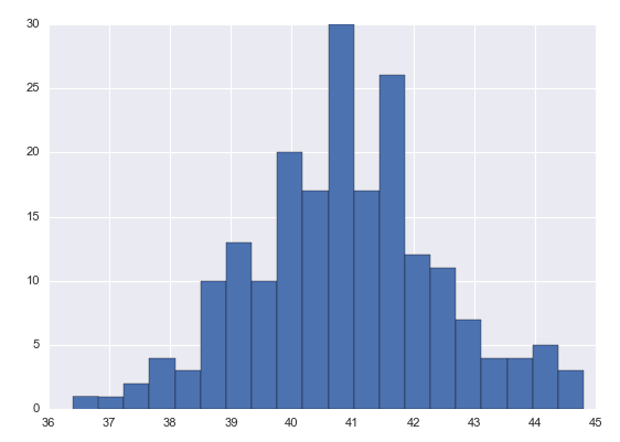
Let's reuse the previous example to explain it. In that example, we resample the original data and derive 200 Bootstrap samples. For each resample, there exists a mean and therefore they constitute the distribution of \bar x* (see the figure below).
The percentile method says to use the distribution of \bar x* as an approximation to the distribution of \bar x. As a result, we only need to find the 0.1 and 0.9 critical values from this distribution and they are the boundary of the CI for μ. In this example, the two values are 38.9 and 43, respectively. The confidence interval for μ by using the Bootstrap percentile method is therefore [38.9, 43].
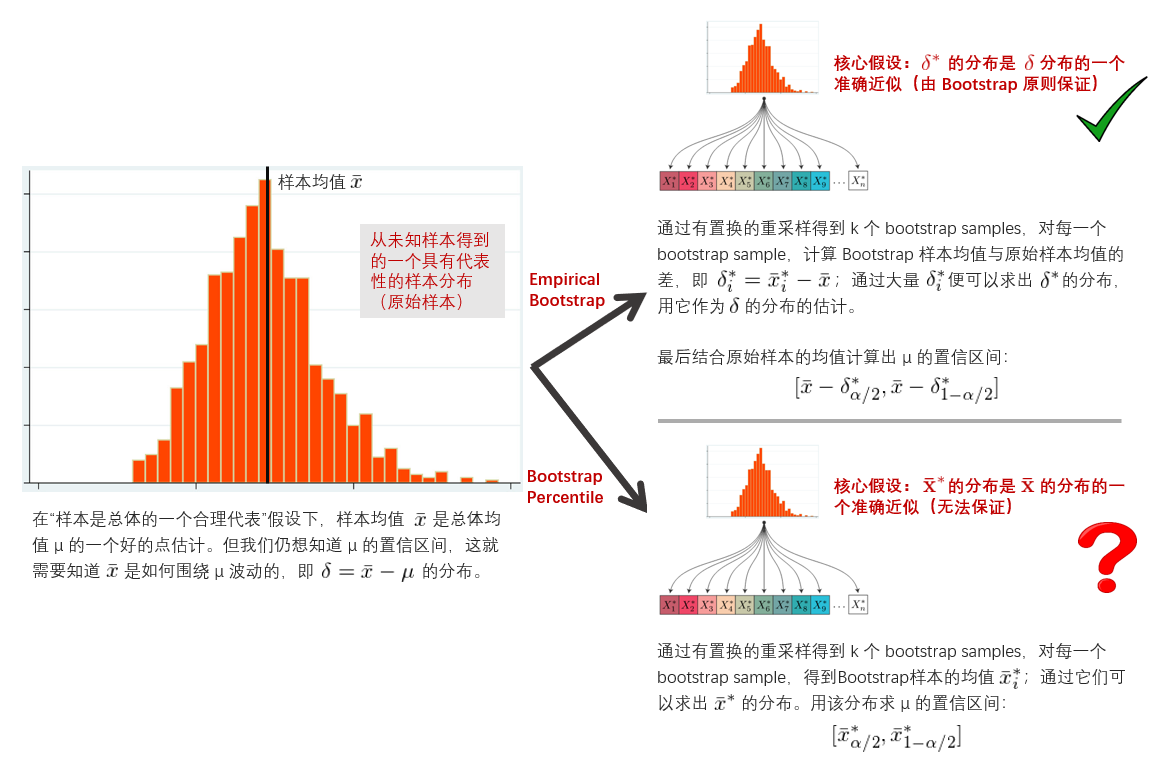
It becomes very clear that the CIs computed using these two approaches are not the same. Is one better than the other? The difference between the empirical Bootstrap method and the Bootstrap percentile method can be summarized as follows. Empirical Bootstrap method approximates the distribution of δ using that of δ*. It then adds the error to both sides of the sample mean. As a result, the confidence interval is centered at \bar x. Bootstrap percentile method approximates the distribution of \bar x using that of \bar x* (since we only have one sample from the population, we do not have the distribution of \bar x, and this method says we can use the distribution of \bar x* as a good approximation). Then the CI comes from the distribution of \bar x* directly. A very strong assumption here is that the distribution of \bar x can be well-approximated by the distribution of \bar x*. However, this cannot be guaranteed, and therefore this method should not be used.
Bootstrap principle tells us the following: the sample statistic \bar x is 'centered' at the population mean μ, and the Bootstrap statistic \bar x* is centered at \bar x. If there is a significant separation between \bar x and μ, then the distributions of \bar x and \bar x* will also differ significantly (i.e., the assumption of the Bootstrap percentile method fails to hold). On the other hand, the distribution of δ = \bar x - μ describes the variation of \bar x about its center. Likewise the distribution of δ* = \bar x* - \bar x describes the variation of \bar x* about its center. So, even if the centers are different, the two variations about the centers can be approximately equal. Consequently, we should use \bar x as the center and use the distribution of δ* to find the error. A confidence interval calculated this way is likely to be accurate. The above argument suggests that the empirical Bootstrap method is better than the Bootstrap percentile method. In practice, the former should be used.
The following figure summarizes the difference between the two approaches.
5 Bootstrapped-t method
In addition to the two methods discussed in the previous two sections, we'd like to talk about one more method, the Bootstrapped-t method. As its name suggests, this method is similar to the traditional method. In the traditional method based on Normal Theory, we look up the t-value table to find the critical values for the CI of the mean. It assumes that the distribution of the population statistic is symmetric.
In practice, however, this assumption may fail. In that case, the critical values from the t-value table are incorrect. This motivates the development of the Bootstrapped-t method, which allows asymmetric t values for the CI. The key idea of this method is to convert the statistics of those Bootstrap samples to a set of t-statistic. These many values of the t-statistic will give us a distribution of it. We use this distribution, instead of the t-value table, to derive the critical values required by the CI. The CI is then computed by,

where s_{\bar x} is the standard deviation of the original sample. As for the mean, we can use the following formula to transform the Bootstrap sample mean to a t-statistic (note that if the target statistic is not the mean, it is possible that there exists no analytic expression for such a transformation),

where \bar x*_i and s*_i are the mean and standard deviation of the ith Bootstrap sample, respectively, and n is the sample size. Back to our example, the cumulative density function of the 200 Bootstrapped t-statistic looks like the following.
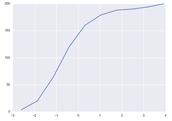
The critical values of the Bootstrapped t-statistic are -1.17 and 1.81. The CI for μ is therefore [31.82, 46.62]. Note that the range of this CI is wider than the CIs calculated using the other two methods. This is because we use the standard deviation of the original sample in this calculation. Since there are only 10 data in the original sample, its standard deviation is huge, and it leads to a wider CI.
6 Not just the mean
For the sake of comparing different Bootstrap methods, so far in this article we have been talking about the population mean as our target statistic. The Bootstrap technique is equally effective to find the CIs for other statistics. Let's use the median as an example. We still have the 10 sample data as before (30, 37, 36, 43, 42, 48, 43, 46, 41, 42) and they come from some unknown population. We will apply the empirical Bootstrap method to find the 95% confidence interval for the median. With those 200 Bootstrap samples, it is straightforward to find the critical values we need. Since we are concerned with the 95% CI, the critical values are the errors corresponding to the 2.5% and 97.5% percentiles, and they are -5.0 and 2.5. In addition, the sample median is 42. Therefore, the 95% confidence interval for the median is [39.5, 47].
7 Bootstrap and quantitative investment
This article explains how to use Bootstrap technique to measure the error in parameter estimation. Bootstrap does not make assumption of the population distribution, and therefore it can be applied to any statistic. This makes it a very powerful tool. It is important to mention that the resampling of Bootstrap can't improve our point estimate. Using the mean as an example, the sample mean \bar x is the point estimate of the population mean μ. By using Bootstrap, we would compute \bar x* for many resamples of the data. If we took the average of all the \bar x* we would expect it to be very close to \bar x (in fact, it can be shown that the expectation of \bar x* equals \bar x). This wouldn't tell us anything new about the true value of μ. However, the values of \bar x* is very effective to help us measure how \bar x varies around μ, and this is the essence of the Bootstrap method.
Bootstrap technique has a lot of useful applications in quantitative investment. For instance, it can be used to correct the parameter estimation bias. Suppose we'd like to know the correlation coefficient of the returns of two assets and the only data we have is time series of historical return. By using the empirical Bootstrap method, we can find the error in the parameter estimation, and this can help derive better investment strategy or achieve more solid risk management. As another example, classification tree is a simple algorithm that can be used for stock selection. It is sensitive to the in-sample data and its prediction has a lot of variances. Bootstrap technique can be viewed as a great ensemble learning meta-algorithm and it can be applied to boost the performance of the simple tree-based classification algorithms. The 'bagging' algorithm, which combines classification tree and the Bootstrap technique, is capable of providing more accurate prediction.
Finally, the methods discussed in this article are all nonparametric, i.e., we make no assumptions at all about the underlying distribution and draws Bootstrap samples by resampling the data. In some problems, if we know the population distribution, we can use the so-called parametric Bootstrap. The only difference between the parametric and empirical Bootstrap is the source of the Bootstrap sample. For the parametric Bootstrap, we generate the bootstrap sample from a parametrized distribution. For example, if we know that the population is exponentially distributed with some unknown parameter λ, we can apply the parametric Bootstrap method to estimate the confidence interval of this parameter. Due to space concern, we are not going to expand the discussion on this topic. The readers are encouraged to go through the relevant reference.
免責聲明(míng):入市有風險,投資需謹慎。在任何情況下(xià),本文的(de)内容、信息及數據或所表述的(de)意見并不構成對(duì)任何人(rén)的(de)投資建議(yì)。在任何情況下(xià),本文作者及所屬機構不對(duì)任何人(rén)因使用(yòng)本文的(de)任何内容所引緻的(de)任何損失負任何責任。除特别說明(míng)外,文中圖表均直接或間接來(lái)自于相應論文,僅爲介紹之用(yòng),版權歸原作者和(hé)期刊所有。


