Brownian motion, Ito's lemma, and the Black-Scholes formula (Part I)
發布時(shí)間:2017-03-09 | 來(lái)源:
作者:石川
1 Introduction
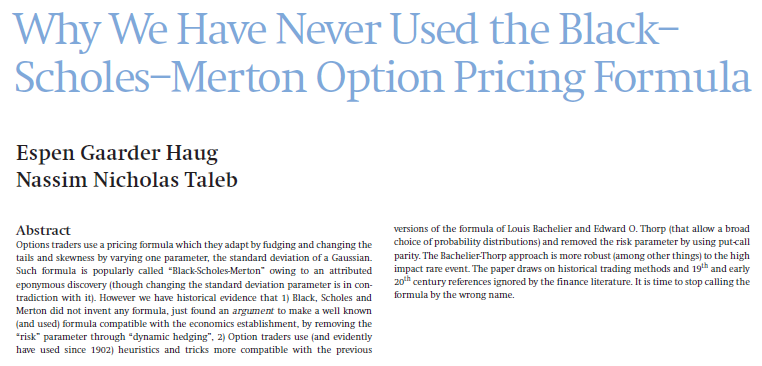
The Black-Scholes formula (also known as the Black-Scholes-Merton formula) for option pricing is very famous in quantitative finance. It is one great example that applies stochastic process to financial instrument pricing. The BS formula related questions are always asked, with no exception, in Wall Street quant job interviews. However, Nassim Nicholas Taleb, the author of The Black Swan despises the BS formula and he even co-authored an article entitled Why we have never used the Black-Scholes-Merton option pricing formula to denounce it.
Different people hold distinct views on how effective the BS formula is in investment practice. My point of view, however, is that the BS formula is just a result; it is a product from the rigorous derivation of stochastic calculus. Looking at the nature of the phenomenon, there is a powerful mathematical system behind it that allows us to quantify the price of stocks, options, and other derivatives using stochastic processes. A familiarity to this analytical approach is essential to those who want to achieve something in the field of quantitative finance.
It is by no means easy to master this mathematical system. If one googles how to derive the BS formula, the concepts such as the Brownian motion, Ito's lemma, and stochastic differential equations will pop up. They are all integral elements of this system, seamlessly linked with each together and perfectly fitted in the framework of stochastic calculus. People who are familiar with this can fully appreciate the beauty of mathematics behind the framework. For people who are not familiar with it, every concept may seem mumbo-jumbo; it is uneasy to figure out the logical relation between them even with higher mathematics knowledge.
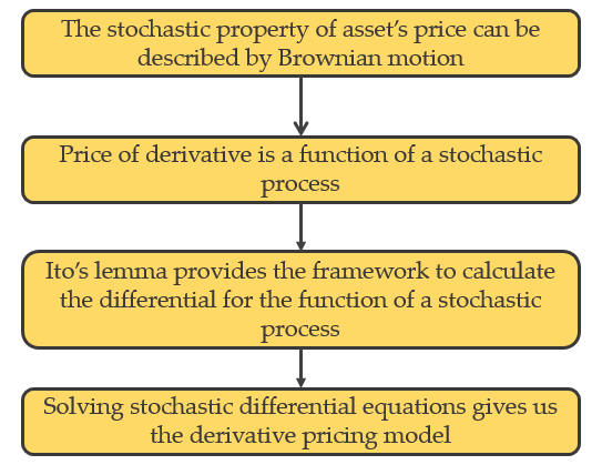
To put it simple, the (standard) Brown motion is the simplest continuous stochastic process. It is the basic model for describing the stochastic nature of asset prices. For options and other derivatives, their prices are functions of the underlying asset price. Since asset price is a stochastic process, the derivative price is a function of that stochastic process. The Ito's lemma provides a framework to differentiate the functions of stochastic process and this is of particular significance to derivative pricing (before Ito's work, people did not know how to do it). Ito's lemma allows us to derive the stochastic differential equation (SDE) for the price of derivatives. Solving such SDEs gives us the derivative pricing models. The derivation of the BS formula is one simple example of this procedure.
Given the importance of stochastic calculus, we plan to talk about it in a series of two articles. As the first part, today's article will explain the Brownian motion and its properties, as well as present the basic form of the Ito's lemma. We tried hard to reveal the properties of the Brownian motion and its implications to stock price movement. In the second part of this series, we will start with a more general form of the Ito's lemma, and apply it to solve for the geometric Brownian motion, and finally derive the BS equation and the BS formula.
We hope that these two articles will provide you an intuitive understanding about the mathematical framework of stochastic calculus, and help you appreciate the beauty of mathematics where different elements seamlessly connect with each other to derive an elegant pricing formula.
2 Brownian motion: Development and mathematical definition
In 1827, while looking through a microscope at particles trapped in cavities inside pollen grains in water, Scottish botanist Robert Brown noticed the random motion of the particles; but he was not able to determine the mechanisms that caused this motion. Albert Einstein published a paper in 1905 that explained in precise detail how the motion that Brown had observed was a result of the pollen being moved by individual water molecules. The development of Brownian motion in physics has been improving since then.
As a contrast, its development in mathematics is slower. The precise mathematical definition of the Brownian motion was not developed until 1918 by Norbert Winner. Therefore, the Brownian motion is also referred to as the Wiener process. The Brownian motion is a continuous-time stochastic process, or a continuous-space-time stochastic process. It is a stochastic process for which the index variable takes a continuous set of values, as contrasted with a discrete-time process for which the index variable takes only distinct values.
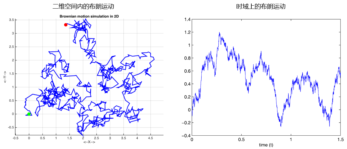
The figure above shows two examples of the Brownian motion. The one on the left is a two-dimensional Brownian motion where the two axes represent the space domain, while the one on the right is a one-dimension Brownian motion and the x-axis is the time domain. The Brownian motion on the right looks very similar to the movement of stock price, and this motivates people to use it to model stock price. The first person who considered this process is Bachelier, who used Brownian motion to evaluate stocks and options in his Ph.D. thesis entitled Théorie de la spéculation in 1900.
The one-dimensional standard Brownian motion is defined as follows: There exists a probability distribution over the set of continuous functions B: R -> R satisfying the following conditions:
1. B(0) = 0,
2. (Stationary) for all 0 ≤ s < t, the distribution of B(t) - B(s) is the normal distribution with mean 0 and variance t - s, and
3. (Independent increment) the random variables B(t_i) - B(s_i) are mutually independent if the intervals [s_i, t_i] are nonoverlapping.
We refer to such a process B(t) as the standard Brownian motion.
The definition indicates that the Brownian motion starts from some original point at t = 0. In any given finite time interval Δt, B(Δt) satisfies a normal distribution with mean 0 and variance Δt, where the variance increases linearly with time. Independent increment means that the movements of the Brownian motion in nonoverlapping intervals are independent. This is immediately followed by the fact that the Brownian motion is a Markov process, and it implies that the movement after t depends only on the location at t, and has nothing to do with the historical path before t. In other words, the current value B(t) at t contains everything we need to predict the future.
3 Properties of the Brownian motion
Here are some facts about the Brownian motion, and they have important implications to modeling stock price movement using it:
1. The path crosses the x-axis (time axis) infinitely often.
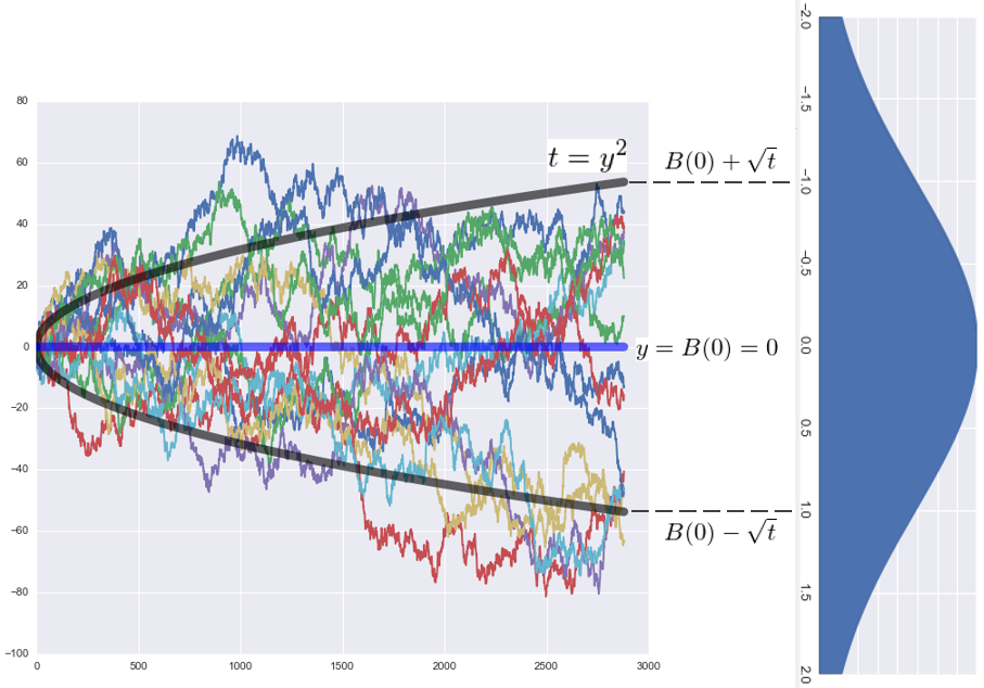
2. B(t) has a very close relation with the curve x = y^2. At any time t, it does not deviate from this curve too much.
3. Let M(t) be max_{0 ≤ s ≤ t} B(t), it can show that Prob(M(t) ≥ a) = 2 × Prob(B(t) ≥ a);
4. It is nowhere differentiable (this is very important).
To explain the first two properties, the following figure shows 15 sample paths of 15 standard Brownian motion in time interval 0 to t. Each path crosses y = 0 (the time axis) multiple times with the exception that only very few paths appear to be on the same side of y = 0 for the entire period. However, they will eventually cross the x-axis as t increases. The black parabola is the curve of t = y^2. We can see that although each sample path shows a distinct randomness, at any time t' ≤ t, they do not deviate too far from the parabola curve which is B(0) +/- the square root of t. On the right of the figure is the probability density function of the normal distribution at t whose mean is 0 and variance is t. The range of the parabola corresponds to one standard deviation above and below the mean of the normal distribution.
Suppose we choose to use the Brownian motion to describe the high frequency intraday price movement (later in this article we will point out that a more accurate model is the geometric Brownian motion with drift, but let's now use the Brownian motion for a short while), then the two properties above mean that the stock price will fluctuate around the open price and as time passes by, it will not deviate too much from the open price +/- the square root of t times the standard deviation of the price. These properties are important to high frequency traders.
The third property shows how to derive the probability model for the extreme values of the Brownian motion. Since B(t) satisfies the normal distribution N(0, t), using Prob(M(t) ≥ a) = 2 × Prob(B(t) ≥ a), we can derive Prob(M(t) ≥ a) easily,
where Φ is the cumulative density function of the standard normal distribution. This can be proved by the Markovian property and the reflection principle. Likewise, let m(t) be the minimum value of B(t) in [0, t], i.e., m(t) = min_{0 ≤ s ≤ t} B(t). It can be shown that
These results can be used to quantify the probability distribution about the extreme values of the stock price, which can be of great importance in risk management. The last property is a crucial nature of the Brownian motion as a stochastic process. It says that although the Brownian motion is continuous, it is not differentiable everywhere (this can be proved by contradiction with the usage of the mean value theorem and the third property). This is very intuitive to understand. Let's take a look at those 15 sample paths of the Brownian motion. Each of them has been fluctuating up and down, demonstrating its randomness. It is clear that the trajectory of the Brownian motion is completely different from any continuous and smooth trajectory that we are familiar with.
The non-differentiability means that classical calculus is useless in analyzing the Brownian motion. This was undoubtedly frustrating because people finally come up with a simple random process (to model stock price), but lacked the tools to further study it. However, the puzzle was solved with the development of Ito calculus. It is no exaggeration to say that Ito calculus laid the foundation of modern financial mathematics.
4 Quadratic variation
For a partition Π = {0 = t_0 < t_1 < t_2 < … < t_N = T} of an interval [0, T] and a continuous function f(t), its quadratic variation is defined as
If f is continuously differentiable in [0. T], then by using the mean value theorem of classical calculus, it can be shown that
This means that as the partition becomes finer and finer, i.e., as max_i {t_{i+1} - t_i} approaches to 0, the quadratic variation of f(t) goes to zero. What if we change f(t) to the Brownian motion B(t) instead? Remember that B(t) is nowhere differentiable. Regarding the quadratic variation of B(t), the following theorem holds: For a partition Π = {0 = t_0 < t_1 < t_2 < … < t_N = T} of an interval [0, T], let |Π| = max_i {t_{i+1} - t_i}. A Brownian motion B(t) satisfies the following equation with probability 1:
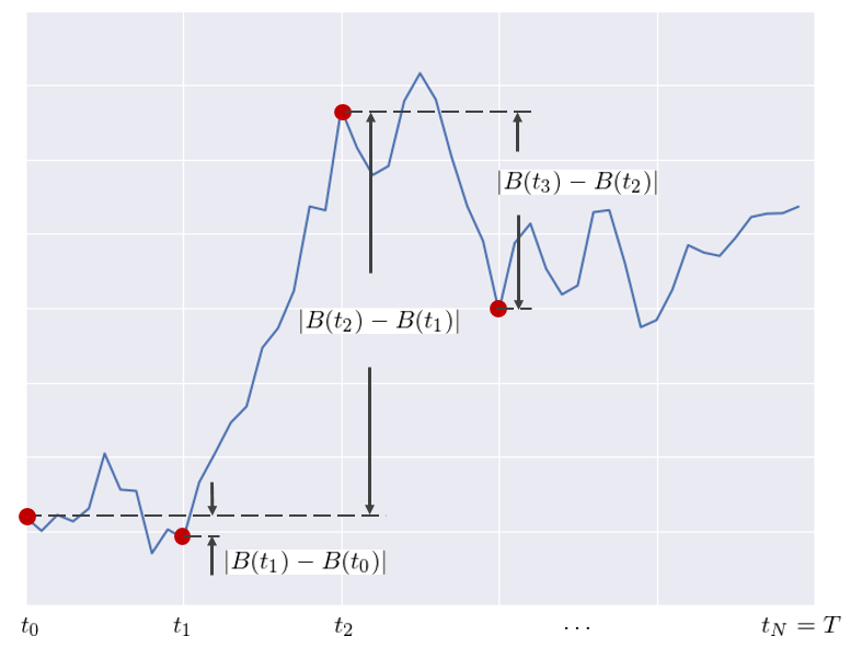
This can be proved by the law of large numbers. It says that as a stochastic process, the quadratic variation of the Brownian motion is T, rather than 0. What does it mean? Consider the following illustration. The blue curve is the path of a Brownian motion, and the red points show the location of B(t) at different partitioning points. Therefore, (B(t_{i+1}) – B(t_i))^2 is the squared difference of the locations of two adjacent partitioning points. The quadratic variation is the cumulative sum of these squared differences.
For a regular function f(t) that is both continuous and differentiable, as the partition becomes finer and finer, its quadratic variation approaches to 0. However, this is not true for B(t) who is continuous but not differentiable. This suggests that the randomness of B(t) makes it vary too much no matter how small a partitioning interval becomes. The cumulative sum of the frustration of B(t) from those tiny small intervals just won't go to 0. Instead, the limit goes to T, which is nothing but the length of the interval! This is a key property of the Brownian motion. The quadratic variation of the Brownian motion can also be written in the infinitesimal difference form:
As we will show in section 6 of this article, this nonzero quadratic variation of the Brownian motion has significant implications in the derivation of Ito's lemma.
5 Geometric Brownian motion model of stock price
Previous section introduces the standard Brownian motion who follows normal distribution with mean 0 and variance t in the interval [0, t]. Now, we add a drift term μt as well as a scaling parameter σ. This leads to a Brownian motion with drift, denoted by X(t) = μt + σB(t). Note that μt is just a function of time and therefore it has no randomness. It is straightforward to see that X(t) follows a normal distribution with mean μt and variance (σ^2)t. In the infinitesimal form, it becomes
This is a stochastic differential equation. It differs from a regular differential equation in that it has at least one stochastic term (in this case B(t)). Note that this is not contradict to the fact that B(t) is not differentiable. Although B(t) is not differentiable everywhere, dB(t) still has a definite meaning. It represents the change of the Brownian motion within an infinitesimal time interval. Even though we now have the Brownian motion with drift, it is still not the best stochastic process for modeling stock price movement. This is because X(t) or B(t) can take negative values as t passes by. However, the stock price cannot be negative. The return of the stock, on the other hand, can be both negative and positive. Therefore, we can use X(t) to model stock returns.
Let S(t) be the stock price, and dS(t) measures how S changes within an infinitesimal time interval. Therefore, dS(t)/S(t) is the stock return in this interval, and we have
This gives the SDE of S(t):
A stochastic process S(t) that satisfies the SDE is called a geometric Brownian motion. People like to use it to model the stock price because:
1. Normal distribution: Empirical evidence shows that the continuous compound return of stock approximately follows the normal distribution.
2. Markovian property: From the property of the Brownian motion, it is easy to see that S(t) is a Markov process, which means that the current stock price at t contains all the information needed to predict the future, and this complies with the weak form of the efficient-market hypothesis.
3. The fact that B(t) and therefore S(t) are continuous but not differentiable agree withs with the actual movement of stock price.
In order to study the stock price using S(t), we must be able to resolve the SDE above and find a close form of S(t). This can be done with the help of Ito calculus, and this is one of the topics in the second article of this series. We close this section by talking about an interesting example of the Brownian motion with drift. Consider some positive real number μ and let X(t) = μt + B(t). Since the expectation of B(t) is 0, then the expectation of X(t) is E[X(t)] = μt. What we want to figure out is as time passes, which term will dominate X(t)? In fact, it can be shown that X(t) is dominated by μt. For all fixed ε > 0, after long enough time, X(t) will always be between the lines by y = (μ – ε)t and y = (μ + ε)t.
What does this example tell us? It implies that if we believe that the stock market will rise in the long run, i.e., μ > 0, then we should gladly accept any short-term fluctuations it may have and hold the stocks (i.e., ignoring the randomness of B(T)). For a long time, stock price is determined by μt. I guess Buffett must be a mathematician and he must understand this. With his value investment system, he earned a long term drift rate of μ that is higher than the US stock indexes. This allows him to earn stable excess return over the years.
6 Ito's lemma
The Brownian motion allows people to study stock prices. However, as for financial derivatives, their prices are functions of the underlying assets. Let f(B_t) be a continuous and smooth function of the Brownian motion B_t. In financial mathematics, an important topic is to study how f(B_t) changes within an infinitesimal time interval, i.e., the properties of df. As we will show shortly, classical calculus is useless in analyzing df, but the Ito calculus proposed by Japanese mathematician Itō Kiyoshi effectively resolves the issue and that lays a solid foundation for stochastic analysis.
Let's see why classical calculus does not work first. To find df, where f is a continuous and smooth function of B_t, we apply the chain rule:
Since B_t is not differentiable, the differentiation dB_t/dt does not exit. Hence, the formula above makes no sense. Our first try failed. One possible way to work around this problem is to try to describe the difference df in terms of the difference dB_t, rather than dB_t/dt. We have mentioned previously that dB_t has a clear meaning and it is the change of B_t in an infinitesimal time interval. We therefore have
This new formula at least makes sense since there is no need to refer to dB_t/dt which does not exist. In this expression, both f'(B_t) and dB_t can be computed. Unfortunately, this does not quite work. Our second try failed again. To see why, consider the Taylor expansion of f(x) and it gives:
When Δx approaches to 0, the significant term is the first term f’(x)Δx and all other terms are of smaller order of magnitude, which can be ignored. Therefore, df = f’(x)dx is correct. However, is this true for x = B_t? The answer is No. For x = B_t we have
Again, the first term f'(B_t)ΔB_t is still significant. But can other terms be ignored comparing to it? The answer is no due to quadratic variation, which says (dB)^2 = dt. Since the quadratic variation of B_t is not 0, the second term is no longer negligible. The theory of Ito calculus essentially tells us that we can make the substitution (dB)^2 = dt, and the remaining terms are negligible. Hence, the equation above becomes
It is the basic form of Ito's lemma. More generally, consider a smooth function f(t, x) which depends on two variables. In classical calculus, we will get
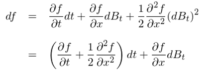
With x replaced by B_t and according to Ito calculus, we have
Comparing the results above shows that, given the nonzero quadratic variation of the Brownian motion, to find df we must add an extra term to the results derived by classical calculus. This extra term is the second order derivative of f to B_t (if f depends only on B_t) or the partial second order derivative of f to B_t (if f depends both on B_t and t). This conclusion changes everything and it permits the usage of calculus in the field of stochastic process.
In the next article of this series, we will apply Ito's lemma to solve the geometric Brownian motion and to derive the BS formula for option pricing.
7 Summary
The Brownian motion is effective in describing the movement of stock price. Its Markovian property agrees with the weak form of the efficient-market hypothesis. By using the reflection principle, it is easy to calculate the probability that the Brownian motion reaches some extreme value within a given period of time, and this is crucial to risk management. To take it further, a more precise model for stock price is the geometric Brownian motion with drift. In the long run, stock price is controlled by the drift rate, and it implies that we should adhere to long-term value investment while ignore the short-term volatility of the stock price called by randomness.
On the other hand, although it is continuous, the Brownian motion is nowhere differentiable. This meets with people's expectation that stock price varies a lot. In financial mathematics, it is important to analyze how the function of a stochastic process changes within an infinitesimal time interval. However, quadratic variation makes classical calculus useless. Ito Kiyoshi proposed a variant of classical calculus, the Ito calculus. It takes into account the quadratic variation of the Brownian motion, and provides a mean of using calculus framework to analyze stochastic process and its functions. This is the foundation of modern financial mathematics.
免責聲明(míng):入市有風險,投資需謹慎。在任何情況下(xià),本文的(de)内容、信息及數據或所表述的(de)意見并不構成對(duì)任何人(rén)的(de)投資建議(yì)。在任何情況下(xià),本文作者及所屬機構不對(duì)任何人(rén)因使用(yòng)本文的(de)任何内容所引緻的(de)任何損失負任何責任。除特别說明(míng)外,文中圖表均直接或間接來(lái)自于相應論文,僅爲介紹之用(yòng),版權歸原作者和(hé)期刊所有。

